Kriging Module

Overview

The kriging module allows to deform the PIPER model or the full FE based to a set of source and associated target control points. More generally Kriging is an interpolation method commonly used to deform geometrical models (along with Radial Basis Function, RBF and Moving Least Square MLS, Jolivet et al., Stapp 2015). Kriging has a lots of similarities with RBF (cost, ability to relax the transformation, etc) and with specific parameters, the formulations are equivalent.

The deformation proposed is based on Dual Krigging formulation with generalized covariance (3D Euclidian distance) as detailed by Trochu (F. Trochu: “A contouring program based on Dual Kriging interpolation”, Engineering With Computers, Vol. 9, pp. 160-177, 1993).

The implementation that is proposed aims to help a number of issues related to Kriging:

• size of the problem: Kriging typically becomes challenging in terms of computing costs when the number of control points becomes large (e.g. over 20000, size of the square matrix to invert). The implementation uses an automatic moving box strategy allowing to use arbitrary numbers of control points (e.g. up to 300000 tested) without noticeable effect on the results.
• cost: several approaches are used to reduce the computing cost. First, the process is parallelized then a sampling strategy is used to select and remove control points which affect the least the interpolation (hereby reducing the computing time without affecting widely the result). The downsampling parameters are accessible by the user.
• distance formulation: the interpolation can use a surface distance instead of an euclidian distance to drive the scaling. This is especially relevant for regions that are close in the euclidian space (e.g. arm and torso) but far away on the skin surface (and anatomically independent). It is based on an approximation of the geodesic distance on a surface and can be used to improve the realism of the skin. The formulation used by Piper is the Biharmonic Distance (Yaron Lipman, Raif Rustamov, Thomas Funkhouser: "Biharmonic distance", ACM Transactions on Graphics 29, issue 3, 2010). Piper uses the "approximate distance" formulation, which uses only a small subset of eigenvalues of the linear system that is being solved to compute the distance. The "Topological distance precision" parameter in Module parameters can be modified to change this number of eigenvalues - it is computed as [the parameter value] / [number of nodes].
• to scale independently the skin, the bones, and then use their surfaces to scale the whole model (called dense scaling in the application).
• change as estimate the relaxation parameter (called nugget) globally or depending on the variability of the interpolation field in a zone and the relative motion of the bones and skin.

Combined, this provides the user a flexibility and adaptability not typically found in existing "morphing" approaches (publications are in preparation). The same approaches are also used to smooth the transformation field.

Description

• Parameters: None
• Metadata:
  • Required: None
  • Optional: Control points defined on HBM
• Target Input: target of type ControlPoint
• Target Output: target of type ControlPoint
• Outputs:
  • a deformed model according to control point and associated target points using Kriging.

Next figure illustrates the Kriging Module GUI, composed of three set of tools:

1. Control points tools to define Control Points and Target Points
2. Deformation Tools
3. Display

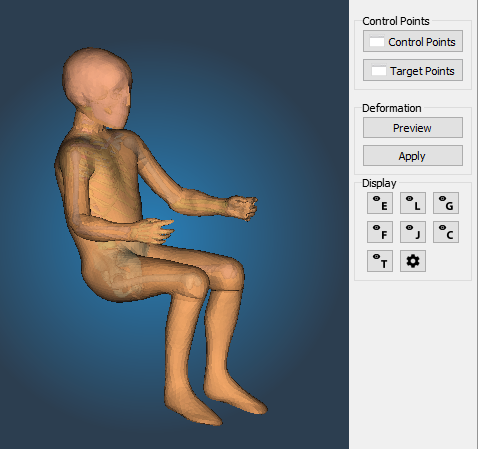
Kriging Module GUI Overview

Control Points

Select set of Control Points to be used for the Kriging deformation. The name and the number of control points of the control points set is displayed.

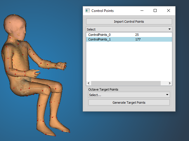
Control Points module tool

A set of control point coordinates can be imported from a text file:

Example of control points file:

-163.87512 -188.34157 -497.91904
-163.87512 188.34157 -497.91904
-249.919373518425 0 -231.471675832181
-48.5283182585665 0 -325.381867183739
-168.1071016685 -170.31156382101 -269.621364726814
-168.1071016685 170.31156382101 -269.621364726814
....

To generate target points associated with the current set of control points, a octave cript an be defined (TODO: describe octave API for script)

Target Points

Select target points existing in the project and define the association with a set of control points.

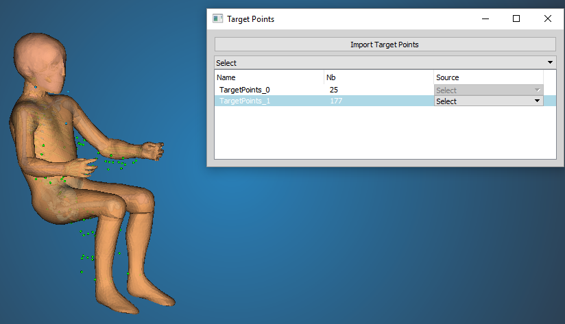
Target Points module tool

A set of target point coordinates can be imported from a text file:

Example of target points file:

-163.87512 -188.34157 -497.91904
-163.87512 188.34157 -497.91904
-249.919373518425 0 -231.471675832181
-48.5283182585665 0 -325.381867183739
-168.1071016685 -170.31156382101 -269.621364726814
-168.1071016685 170.31156382101 -269.621364726814
....

For each target point set, select the control point set to define the deformation. The number of control and target points should match, otherwise an error occurs during deformation. Control points should not be duplicated - duplicates will be automatically removed.

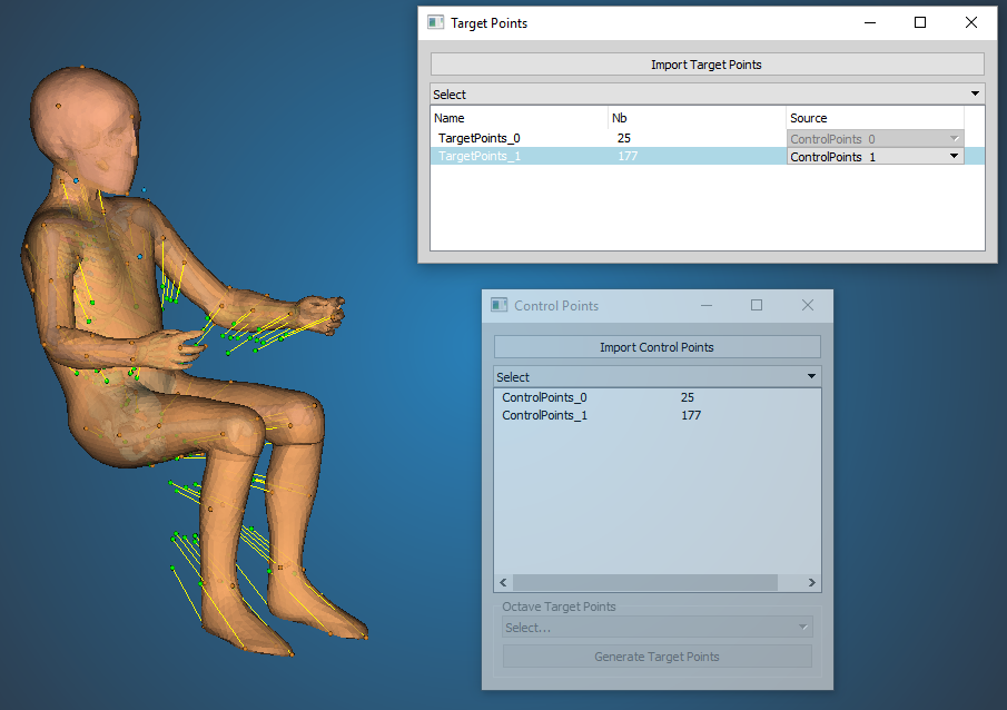
Associate Target Points with Control Points

Deformation Tools

To apply the deformation, open the "Perform Deformation" tool window. There are two modes available: kriging with or without intermediate targets. On the very bottom of the tool window there are two "Apply - ..." buttons, one for each of the modes. Clicking them will deform the loaded HBM model and create a new history node for it (see Model History menu).

Kriging with intermediate targets

Kriging with intermediate targets does not use the input control points to directly deform the entire model, but rather to create two intermediate targets - one for skin and one for bones. This means that only nodes of entites marked as skin in the anatomy database (see "entity" element) will be deformed separately and so will nodes marked as bone. Results of this deformation are temporarily stored and used as the intermediate targets, i.e. all nodes of bones and skin are used as control points, with targets defined by the input set of control points.
There are numerous options that allow for different workflows when the intermediate targets are used. The following list describes them as they are placed in the tool window, top to bottom:

• Skin target options:
  • Topology-aware distance: This allows toggling the distance formulation as discussed in the Overview. Computing the topology-aware distance will take usually around 10-30 seconds, but in some cases may significantly improve the result and also, once it is related only to the source, so until it changes (model changes, control points are added or removed), it does not have to be recomputed again for different targets.
  • Used for skin threshold: Only nodes that have the "use for skin" (see Skin/bone association) parameter equal to or higher than this threshold will be used to create the skin intermediate target.
  • Preview: A preview of the skin after kriging can be visualized as a semi-transparent red surface (see the Figure below). Note that neither selection, blanking or quality computation are possible on the preview surface - it is intended only to provide a quick overview. Changing any parameters relevant to the deformation, such as position of target points, will automatically disable the visualization. Upon ticking the preview box again, it will recompute it using the updated input.
    

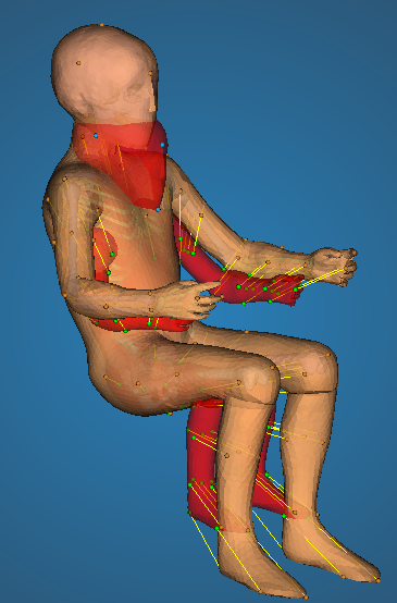
    Deformation Preview
• Bones target options:
  • Used for bones threshold: Only nodes that have the "use for bones" (see Skin/bone association) parameter equal to or higher than this threshold will be used to create the bones intermediate target.
  • Fix bones: Enabling this option will prevent any nodes that belong to bone entities to move during the deformation. Note that they will still be used as control points in order to constrain the movement of the surrounding flesh, but their position will not change, even if some nugget is assigned to them.
  • Preview: Bone preview is visualized as a semi-transparent yellow surface. It behaves the same way as the skin preview (see description above).
• Decimation: In order to decrease the computation time of the deformation, an automated algorithm for control points decimation is employed. For each control point on the intermediate target (i.e. each node of the intermediate target), a deviation of that nodes source to target displacement from the distance-weighted average of displacement of all surrounding nodes is computed. If that deviation is lower than a specified threshold, the node is considered to be insignificant - it's surroundings describe the same motion, so it is not needed - and will not be used for the kriging. The following list describes the options for this tool:
  • Influence radius: the aforementioned surroundings is a sphere around the node that is being processed. This parameter describes how large that sphere is. Note that even though there is no button to explicitly turn off the automated decimation, setting the radius to 0 will effectively do it.
  • Maximum deviation: this is the deviation threshold. Here deviation means the distance between the actual target and the target that would be obtained if the processed point used the average displacement.
  • Decimate control points: pressing this button will do the decimation. Note that this is useful only for the visualization - upon pressing the "Apply" deformation button, the decimation will be done anyway if it wasn't done already.
  • Visualize control points on intermediate targets: after decimation, the remaining control points can be visualized as blue spheres on the preview of intermediate targets (the preview has to be turned on).
• Automatic nugget computation: There are currently three ways to set the Nugget of control points: define it in the input files (see "Control Points" element), use the default nugget, or use the automatically computed nugget. The automatic computation works on the same principle as the decimation algorithm described above - if all points in the vicinity of a given control point "move the same way", it is not needed. But in the other case, where points in close proximity have very different displacements, high nugget will probably be needed to avoid penetrations and other artifacts. The nugget is therefore set based on the deviation from the average displacement in a given surrounding of each point. Several parameters, described in the list below, are introduced in order to scale this result.
  One difference between the look-up of surrounding between the decimation and nugget algorithms is that the decimation algorithms searches for points that are close to the other point in terms of their source positions, while the nugget uses the target positions instead. The assumption that led to this arrangement is that the most common type of artifact that can be removed by an appropriate nugget is penetration of elements. Therefore, it is more important to track points that are close to each other after the deformation which can signify a potential penetration. Of course, if the penetration is larger than the influence radius, the penetration will not be discovered.
  Note that this feature has not been tested thoroughly yet and probably will work as intended only in some cases.
  • Influence radius: raidus of a sphere around the processed point to consider as surroundings.
  • Skin scale: The computed nugget will be multiplied by this number if it belongs to a skin node.
  • Bones scale: The computed nugget will be multiplied by this number if it belongs to a bone node.
  • Bone-skin distribution ratio: this parameter allows to enforce the constraints defined either on skin, or bone. The average displacement is computed separately for nodes in the surroundings that belong to bones (DEVb) and separately for those that belong to skin (DEVs). The nugget is then computed using this parameter (DISTR) as: Nugget = DISTR * DEVb + (1 - DISTR) * DEVs. For example, setting it to 0 means only deviation from skin will be considered in setting the nugget, effectively saying that displacement of bone is not relevant and should be suppressed, while displacement of skin should be respected. If the processed point is a skin point itself, it will therefore be assigned no nugget, because it will have similar displacement as the average of skin nodes displacement, whereas bone node will have a different displacement and therefore will be assigned a high nugget.
  • Compute nuggets: this will perform the computation. As with the "Decimate control points" button, this is relevant only for visualization - the computation will be done before the final Kriging deformation whether this button was pressed or not. If you don't want to use this option, check the "use default nugget".
  • Visualize nuggets: once the automatic nugget is computed, it can be visualized on the preview surfaces (they must be enabled). The nugget is visualized on a continuous scale from 0 to the highest (negative) nugget value by transition of blue to red color, respectively. As of current Piper version (1.0.0), there is no visualization of the numerical values of the scale, only the highest nugget is written in the console. If decimation was performed, points that have been decimated obviously have no nugget, so they are assigned white color.
• Intermediate target selection: In some workflow, it will be better to use only one of the intermediate targets to transform the model. Either one can be disabled using the check boxes on the bottom of the tool window.

Skin/bone association

These two parameters express how much should a given control point affect bone or skin entities. It is a number between 0 and 1, where 0 means the point does not affect skin/bone at all and 1 is interpreted as "is an actual point of point/skin". This enables to have plausible deformation for both intermediate targets without introducing artifacts coming from control points that are too far away from the points they deform (e.g. control points for spine affecting the skin etc.).

Domain decomposition of HBM

Although some artifacts of the deformation can be mitigated by using the aforementioned tools, there can still be issues in some scenarios. Namely, when several significantly different constraints (control points' targets) are used, the resulting deformation field might be different from what is needed: Kriging will always try to create a single, smooth interpolation based on the provided constraints. Imagine a simple 2D example: let's assume two control point sets, points A and left of them points B, relatively close to each other. Points A move right, away from points B while points B remain stationary, i.e. their target position is equal to their source position. If a single smooth interpolation is defined based on these control points, then on the right side of points B, this interpolation will be represented by a displacement proportional to the displacement by which points B are moved. But since points B do not move, i.e. their displacement is zero, the deformation field on the left side of points B will be a displacement in the opposite direction. This will often not be intended, in fact, the non-moving constraint is probably intended as "everything behind it should also not move" - but that will not be the case in a single smooth field is imposed on the area.
To mitigate this drawback, it is possible to decompose the model into "domains", i.e. areas that are expected to move in a uniform way so that the assumption that the deformation can be represented by a single smooth deformation field is more or less upheld. For most cases, it will be beneficial to decompose the model into parts that are individually, i.e. at each major joint. To minimize the effort needed to do this decomposition, the only metadata that needs to be defined is a set of nodes that create a closed polyline on the skin of the model. This polyline represents the boundary between two domains. Any number of such boundaries can be defined. Piper will subdivide the model into domains and perform kriging on each domain separately and in the end assemble the results back as a single HBM.
To define the boundary point sets ("rings"), use Named Metadata following these rules:

• The name can be an arbitrary string ending with "_decomposition". For example, "Left_arm_decomposition", "Left_knee_decomposition" etc.
• Each ring must be made of nodes that are on the skin, i.e. are part of entities that are defined as skin in the anatomy database (see "entity" element)
• Each ring must form a closed polyline, i.e. for a ring with N nodes, there exists exactly N edges and each node has exactly two neighbors among the other points on the ring to which it is connected by those edges. However, the nodes do not have to sorted in any particular order in the input file.
• Each edge in the ring must be manifold and non-boundary, i.e. exactly two elements must share that edge.

Rings that do not follow the aforementioned rules will simply be ignored (a warning will be written in the Piper console).
This option can be turned off with a check box on the bottom of the tool window. If it is turned on and the required metadata are not present in the model, the option will be ignored and the transformation will be perfomed as if the option was turned off.

Direct Kriging

The "direct" kriging does not use any preprocessing of the control points - the loaded control points are directly used to define the deformation. In case there is only a small amount of control points (relative to the number of the model's nodes), it will likely lead to some artifacts. For this reason, direct kriging should be used only for a dense network of control points or in conjuction with some model specific knowledge. For other cases, the Kriging with intermediate targets should be preffered.
Note that even though the intermediate targets will not be used for Direct Kriging, one can still use the previews of intermediate targets to get a fast assessment of the effects of the deformation.

Nugget

A nugget is a "relaxation weight" one can assign to a kriging control point. I represents the uncertainty (variance) of the target position for a given point. A non-zero nugget will allow the control point to violate the target position by at most the nugget value distance in order to make the global transformation more smooth. It is useful in situations where it is not necessarry to follow the target perfectly.
You can specify a global nugget in the Module parameters menu. This value will be used for all control points for any PIPER tool that utilizes kriging (e.g. the Kriging module or the scaling tools in Anthropometry module), unless the nugget is explicitly specified to some other value, as it is for example in the Transformation smoothing tool or by the control points definition when imported from a file. The default value is 0, meaning the target positions of control points will be maintained perfectly.

Display

TODO?