|
PIPER
1.0.1
|
|
PIPER
1.0.1
|
After some transformations (positioning in particular), it is frequent that the element quality is degraded compared to the original model. This can occur on the surface or inside the mesh (3D elements) and it can lead to inverted elements (negative volume or negative jacobian) which prevent the simulation from starting. This module provides different tools to try to help with this problems.
First, the element quality needs to be assessed. There are many metrics and definitions used to define element quality depending on the FE solver and pre-processor. It is assumed that the user can always export the HBM and to compute its favorite quality metrics in another pre-processor (which PIPER does not aim to replace). Within PIPER, two libraries are used to compute quality metrics:
They will provide results different results. In both cases, the variation of element quality (before and after transformation) can be computed which can be helpful to detect problematic regions for smoothing and assess the quality of the transformation (independently from the quality of the original model).
Then to try to improve the quality, three methods are provided. Their principles are summarized below:
Overview of the smoothing methods
| Method | Applies to | Strength and usage scenario |
|---|---|---|
| Mesquite Mesh optimizer | 3D mesh (inside) | Optimize mesh. Use alone or after the others. |
| Surface smoother | Surface mesh | Local defects (on skin). Use first. |
| Transformation smoother | All (not mesh aware) | Minimize distortion without generating penetrations. Use second. |
All three methods can be applied even if the model transformation was not made in PIPER (the transformation smoother can smooth between two arbitrary models).
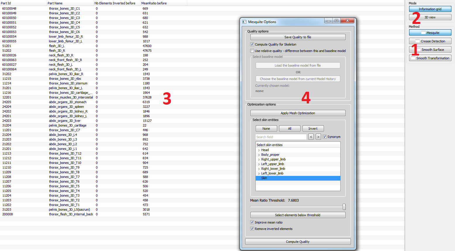
There are currently four different methods available in this module. Only one can be active at a time. To switch between them, use the buttons in the right panel, marked by number "1" in the Figure Module Main Window. Clicking them will also open a window with options of the given method. See below for details on the individual methods.
The results display has two modes - information grid and 3D view. The mode can be changed using the two buttons on the right panel marked by number "2" in the Figure Module Main Window.
The information grid mode is currently used only by the MESQUITE Quality metrics method. It displays the amounts of low quality elements in individual parts of the FE model as text.
The second mode switches to a standard 3D view of the model. Most of the quality methods have a way to mark the low quality or otherwise interesting elements in the 3D view. Also, standard 3D view tools such as metadata showing/hiding, picking etc. are of course available in this mode and can be used e.g. to select which parts of the model to apply a mesh optimization to.
Hint: Most of the mesh optimization methods work with the entire, "full", model (including all nodes and elements). The visualization of finite element model will therefore be activated by default and the entity visualization (PIPER model) automatically switched off. If needed, you can switch it back via the "Display -> Entity" window, using the checkboxes on the bottom of the window. But keep in mind that if you have both modes turned on, you will likely see the model twice, once as a full model, once as entities.
The VTK toolkit integrates quality metrics defined in the Verdict Library. The metrics are computed on 2D and 3D elements (pyramid and penta element metrics are not available in the Verdict Library).
These metrics are not used for any optimization. It is possible to display them in every module that utilizes the 3D view. You can bring it up using the "Element Quality" button in the right panel.
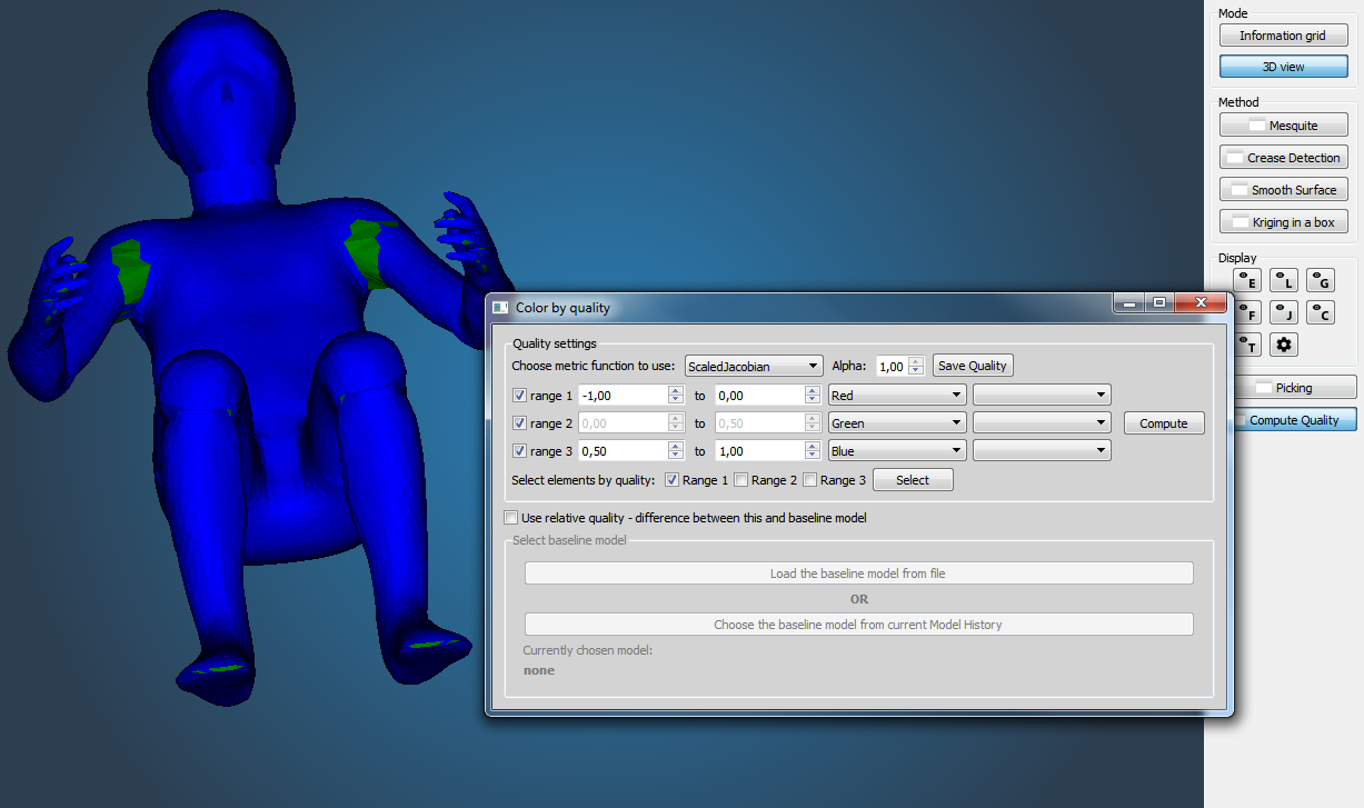
Figure Color by Quality shows the options window for this method. You can choose from a number of quality metrics and set-up up to three quality ranges, each of which will be colored by a different color scheme. Upon pressing the "Display" button, the quality will be computed for each element for which the metric is defined and the elements will be colored. You can save the results to a file using the "Save Quality" button.
Setting up the ranges is simple - tick a checkbox for each range you want to use, then enter the desired thresholds. The extremes of the ranges will be automatically modified so that no two ranges overlap.
The two comboboxes after the range values are used to set up which color will be used with which range. By default, as in the Figure Color by Quality, only the first combobox has some value. In such a case, each element that belongs to this range will be colored by this value. If you specify a second color of the range, the color associated with the element will be a linear interpolation of the two colors. E.g. if you specify a range from 0 to 1 and set colors from green to red, an element with a quality 0.5 will be yellow.
Hint: you can easily create a range that goes from dark to light tones of your favourite color. Simply specify black as the second color to create a range that goes darker with increasing values, or white to create a range that grows lighter. Or use your color as the second one and white/black as first for a similar, yet different effect.
To select elements within some range, use the "Select" button. The checkboxes next to it let you specify which range to include in the selection. Note that using the selection, the 3D viewer automatically switch to rendering the elements based on the selection, not based on the quality, i.e. you will see selected elements in green color, deselected in white. You can then click the "Compute" button again to switch back to coloring the elements by the quality, but the selected elements will remain selected (only not "highlighted").
If you check the "Use relative quality" checkbox, you can specify a "baseline" model, i.e. a different version of your current model (the node and element counts must match!), e.g. before some deformation. You can either specify the model from file or from the Model History, i.e. use the version of the model before you applied some other PIPER operation on it. The quality will then be computed as a difference between the quality of the current model and the baseline one. This way, you can easily see if the deformation you created increased or decreased the element quality of the model.
MESQUITE Quality metrics are defined on 2D and 3D elements but only 3D elements metrics are considered in this module. Inverse mean ratio metric and untangle Beta metric (to detect inverted elements) are computed.
To perform a quality analysis using Mesquite, the user has to:
Results of the quality evaluation are presented in a table with each line corresponds to part defined in the Finite Element Model and the following columns:
The button "Save Quality" export the quality metrics for all elements of the model.
The button "Apply Mesh Optimization" launches the optimisation process - see Improving mesh quality using Mesquite metrics
The second part of the Mesquite Options window allows you to perform some mesh optimization. The GUI for optimization is enabled only if quality is computed and up to date - you have to use the "Compute Quality" button before the optimization.
The optimization is applied on each part (list in the table) with elements that not respect quality criteria. When mesh optimization is applied, each part is optimized individually. Nodes at the free surface of the part are defined as fixed nodes. When an element with quality that does not respect a specified criterion has nodes that are used in the entities that make the skin (use the provided "Select skin entities" box to defines which entities belong to skin), these nodes are not set fixed to allow improvement of this element. The criteria to use can be modified in the "Optimization options" part of the Mesquite Options window (see Figure Module Main Window, window labeled by 4), namely you can specify to improve the mean ratio metric and also set the threshold that should be used to determine what is an acceptable quality; and you can specify whether to attempt to remove inverted elements or not (this is only a binary choice with no further parameters).
You can use the "Select elements below threshold" button to perform a selection of elements. If you need to select elements above the threshold instead, simply use the "invert element selection" from the standard Picking menu.
If you specified that you want to use the relative quality in the "Quality options" part of the Mesquite Options window, the value of the mean ratio threshold will also be relative - value of 0 will mean elements that have the same quality both in the current and baseline mesh, negative values will be elements that have lower quality now than in the baseline mesh and positive values mean elements that improve their quality in comparison to the baseline mesh.
The surface smoothing method uses a windowed sinc function interpolation filter to relax the node positions on a surface of an entity (also known as Taubin smoothing). This means that only 2D elements (triangles, quadrilaterals...) will be take into account for the smoothing. Therefore, this method is useful in preprocessing surfaces that you intend to use as targets for Transformation smoothing or similar purposes, or fixing small defects, but will not increase the quality of the model too much in terms of its suitability for FE simulation as problems are often in the 3D elements.
After the smoothing is finished, a new model history is always added, so you can undo the smoothing at will. Apart from starting the smoothing process by pressing the "Smooth surface" button, there are three options you can change in the GUI of the method:
Hint: Note that the filter operates only on selected nodes, not elements! However, if you want to smooth an area that you selected using element selection, you can simply use the "Select nodes of selected elements" button in the "Picking" toolbox to select the appropriate nodes and then run the smoothing. 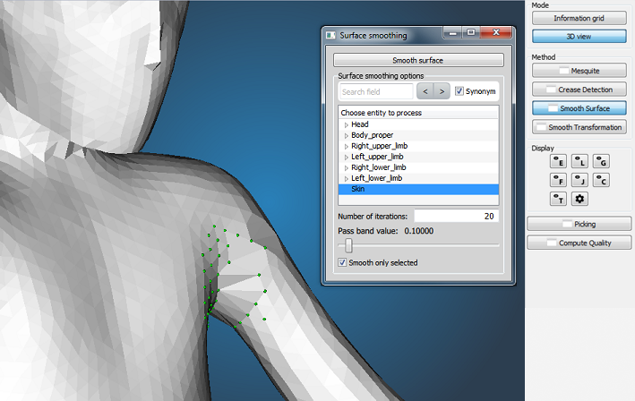

More details can be found in the documentation of the smoothing filter or in the original paper: Optimal Surface Smoothing as Filter Design, G. Taubin, T. Zhang and G. Golub, IBM tech report RC-20404, 3/12/96.
One of the most common types of unwanted deformation that happens to an FE mesh after positioning is that unnaturally sharp creases appear around areas that were bent. This method, which require to specify a baseline model, automatically detects those areas and selects them. It does not have any tool to remove this damage, but the selection can be carried over and used as a target for other optimization methods, such as Transformation smoothing and Smoothing the surface of an entity.
The method uses a simple algorithm that divides the mesh into a set of clusters of elements based on the change of the dihedral angle of elements (the angle between two neighboring elements) before and after a deformation. If the change of dihedral angle between two elements is larger than a specified threshold, each of those elements is added to a different cluster. In the example in Figure Surface crease damage detection, elbow was extended. Ideally, this will put elements in the forearm and the rest of the body to two different clusters, as the change of dihedral angle around the elbow will be large. However, in practice, the positioning methods will likely not be able to create a smooth transition in this area, instead some unnaturally sharp transitions will appear around the elbow, as we can see in the Figure. Using the clustering algorithms, elements that form these sharp transitions will create narrow clusters, only few or even one element "thick", i.e. most of the elements of the given cluster will be on its boundary. This method detects and selects those clusters.
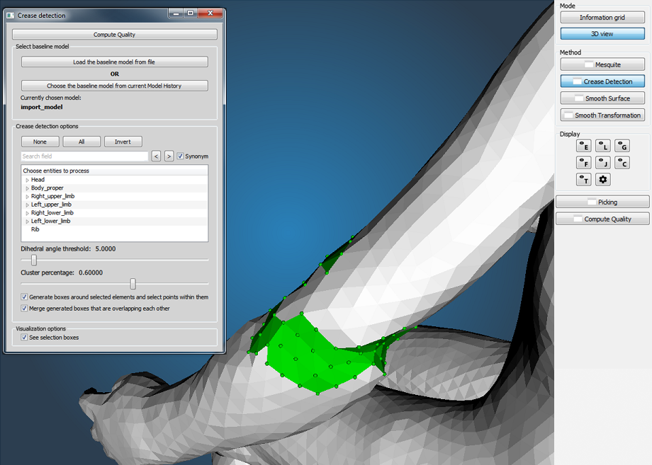
The options window of the crease detection method is divided into these four parts, going from top to bottom (please refer to Figure Surface crease damage detection):
Hint: you can work with the boxes created with crease detector just like with any other boxes you created with the "Picking" toolbox using the box manager inside "Picking" toolbox. 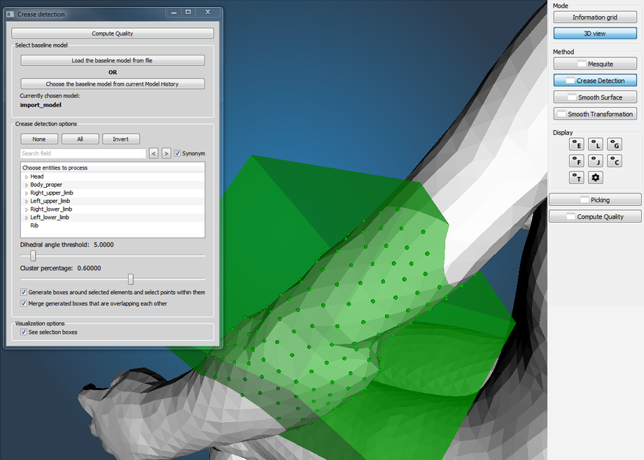
Mesh smoothing algorithms usually smooth the mesh based on some general quality metrics. However, smoothing disconnected groups of elements independently could lead to penetrations between them if the boundary is not kept, and to insufficient correction if it is. In the case of positioning and personalization, the user has access to the mesh before the deformation that potentially caused the damaged (assuming the initial model quality is acceptable). This transformation smoothing method takes this "baseline model" and the target model obtained from positioning or personalization and creates a smooth transformation of the former to the latter. This has the advantage of working with the entire model at once while not generating penetrations (as long as the transformation is smooth). A publication on this approach is being prepared. PIPER currently provides two algorithms to perform this transformation smoothing. One is based on dual Kriging interpolation (see Kriging Module) and the other on averaging local displacements of the smoothed points.
Regardless of the method, the first step is always to select a baseline model (from file or model history; please refer to the Surface crease detection section above for details) as the transformation will be smoothed between the baseline and the current model.
In case of transformation by kriging, the region in which the transformation is smoothed is solely based on selection boxes. You can create the selection boxes manually using the "Picking" toolbox or with the Surface crease detection. When using the "Picking" toolbox, it does not matter whether you are creating the boxes in the node selection or element selection mode - only the boxes themselves will be considered. If you see the message "Smoothing not processed, check if all required parameters are set", it may mean, among other things, mean that there is no selection box.
Hint: check the "See selection boxes" in order to visualize them. Hold CTRL when drawing the box to activate the de-selection mode. This way, nothing inside the box will actually be selected.
Surfaces of entities selected with "Select target entities" are used to constrain the transformation, i.e. taken as a target. This means that nodes on the selected entities will be considered as control points for the kriging (but of course only those that are in a selection box) and all other nodes will be transformed according to them.
Once target entities and selection boxes have been selected, you can start the smoothing by pushing the "Smooth" button. Please note that for larger models and/or selected areas, this action can take up to several minutes.
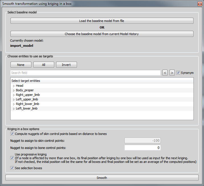
Advanced parameters are related to (1) the "strength" of the smoothing allowed on both parts that are smoothed and on the entities selected for targets ("nugget" parameter), and (2) the strategy to deal with the large amount of control points typically used in the process (computing cost issues). The parameters and options are described below. Experimenting with a small model or region can be helpful to better understand their effects.
The first three lines of controls (see Figure Smooth transformation) serve to set up Nugget of skin control points and bone control points.
WARNING - This method has not been tested thoroughly yet (as of version 1.0.0), it might not work as expected in some cases.
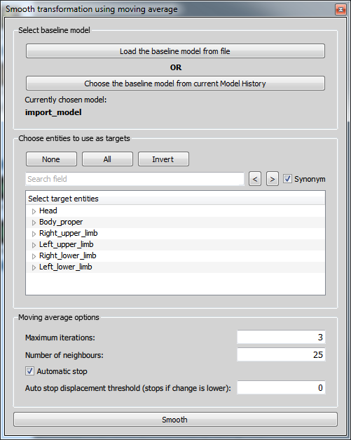
This method smooths directly the displacement of each point that was imposed by the transformation. Points that belong to entities selected as targets are not smoothed. For each other point, a specified number of nearest neighbors (based on the source positions) is found. Then, an average displacement within this neighborhood is computed and the current displacement of the point is replaced by this average. This is done in several iterations. Figure Moving average GUI shows the parameters that can be set:
The moving average method currently works over the whole mesh, so no boxes, as in case of the previous method, are needed.
 1.8.10
